Skip to content

SECTION 03 / 10

Markov’s inequality

On this page 8 headings

Learning goal: Bound a large non-negative value using only its average.

Conditions to check

Markov’s inequality requires a non-negative random variable and a positive threshold.
A bound above 1 provides no improvement over the trivial bound of 1.

The ideaSuppose the average pocket money in a class is ₹50 and nobody can have negative money.
Could half the class have ₹500 or more?
No: those students alone would push the average to at least ₹250.
Knowing only the average already limits how many people can have huge values.
That is Markov's inequality.

Why "concentration inequalities"?

Often we do not know the full distribution of a random variable.
Maybe it is too complicated to compute, or we just don't have it.
We might only know its mean, or its mean and variance.
Concentration inequalities still let us say something useful: they put an upper limit on the probability of a rare, extreme outcome.
Equivalently, they say values usually concentrate near the typical value.

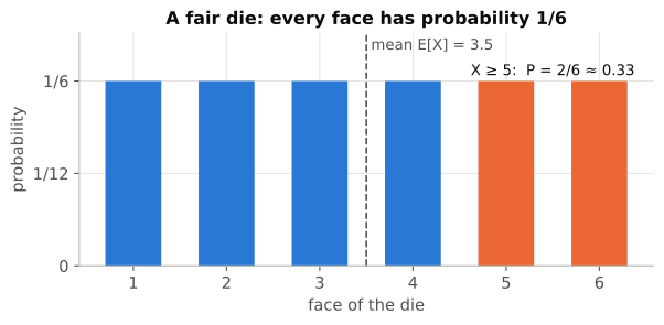
Key statementReview with a die, X = face shown:

Sample space = {1,2,3,4,5,6}; event space = power set of {1,…,6}; probabilities = {1/6, 1/6, …, 1/6}.
$P (X \geq 5) = P (X \in {5, 6}) = 2/6 = 1/3 \approx 0.33$ .
$E [X] = \frac{1 + 2 + \dots + 6}{6} = \frac{21}{6} = 3.5$ .

Bar chart of a fair die, faces 5 and 6 highlighted — The full distribution of a fair die. When we know this, we can compute any probability exactly.

Markov's inequalityFor any non-negative random variable X and any $a > 0$ :

P (X \geq a) \leq \frac{E [ X ]}{a} .

Reading the formula

Left side: the chance of a big value (at least a).
Right side: needs only the average.
The bigger the threshold a, the smaller the bound.
Big values are rarer.
The bound is only useful when $a > E [X]$ .
Otherwise $E [X] / a \geq 1$ , and every probability is already at most 1.

Why it is true: a short proof

Split the average into outcomes below a and outcomes at or above a.
Every outcome contributes something ≥ 0 because X ≥ 0, and those at or above a contribute at least a each:

E [X] \geq x \geq a \sum x P (X = x) \geq x \geq a \sum a P (X = x) = a P (X \geq a) .

Divide both sides by a and you get Markov.
This is exactly the pocket-money argument written in symbols.

Worked example 1: the die

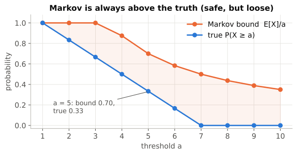
Pretend you only know $E [X] = 3.5$ .

Markov: $P (X \geq 5) \leq \frac{3.5}{5} = 0.7$ .
True value: $\frac{1}{3} \approx 0.33$ .
Since 0.33 ≤ 0.7, the bound holds.
It is loose because it must hold for every non-negative random variable with mean 3.5, not just this die.
Try a = 3: $3.5/3 \approx 1.17 > 1$ .
Useless, as expected, because 3 is below the mean.

Markov bound versus true tail probability for the die — Markov's bound (orange) always sits above the true probability (blue). It is safe but loose.

Worked example 2: k-means

After running k-means, the average distance of a point to its cluster centre is 5.
Your randomised algorithm picks a point at random.
What is the chance its distance is 20 or more?

X = distance, which is never negative, with $E [X] = 5$ and $a = 20$ :

P (X \geq 20) \leq \frac{5}{20} = 0.25.

So at most 25 % of points are "far" (≥ 20) from their centre.
You learn this without looking at a single individual distance.

Worked example 3: your own

A website's average page-load time is 1.2 s.
Markov says at most $1.2/6 = 20%$ of loads take 6 s or more, at most $1.2/12 = 10%$ take 12 s or more, and so on.

Check yourself

Average exam score is 40 (scores are ≥ 0). At most what fraction scored 80 or more?

$40/80 = 0.5$ , so at most 50 %.

Why can't Markov tell you anything about P(X ≥ 2) when E[X] = 3?

The bound is 3/2 = 1.5, which is bigger than 1, so it says nothing new.

Key points to remember

Check that X is non-negative and the threshold is positive.
Divide the mean by the threshold to get an upper bound.
The bound is not an exact probability; a result above 1 is uninformative.

YOUR STUDY PROGRESS

Finished this section? Save your progress.

Back to top ↑