
REVISION AND PRACTICE
Extension: completing the JL proof
On this page 15 headings
Learning goal: Turn a one-vector error bound into a guarantee for all point pairs.
Goal: make a large projection error unlikely
- Start with k independent standard normal coordinates.
- Their squared values add up to a random total S. Its expected value is k.
- We want the chance of S being much larger or smaller than k to be small. Assume .
Step A: get an upper-tail bound
1. See why plain Markov is too weak
Applying Markov directly gives:
- For , this upper bound is about 0.91.
- That allows up to a 91% failure probability, so it is too weak for a useful accuracy guarantee.
- It also does not improve as k increases.
2. Exponentiate before applying Markov
- Choose a positive number λ smaller than .
- The exponential function is increasing. Transforming both sides preserves the event.
Now apply Markov to the positive exponential random variable:
3. Use independence to split the expectation
- S is a sum of independent squared coordinates.
- The exponential of a sum is a product. Independence lets us multiply the expectations.
4. Use the standard Gaussian identity
For a standard normal random variable Z and λ :
There are k identical factors, so the bound becomes:
5. Choose λ to tighten the bound
Minimizing the preceding expression gives:
Substitute this value:
6. Put the result into a convenient form
The logarithm inequality below gives a simpler, slightly looser bound:
- For a fixed between 0 and 1, the failure bound falls exponentially as k grows.
- This is the improvement that plain Markov could not give.
7. Control the lower tail too
Applying the exponential method to the lower tail gives:
This controls a projection that is too small. The preceding upper-tail bound controls one that is too large.
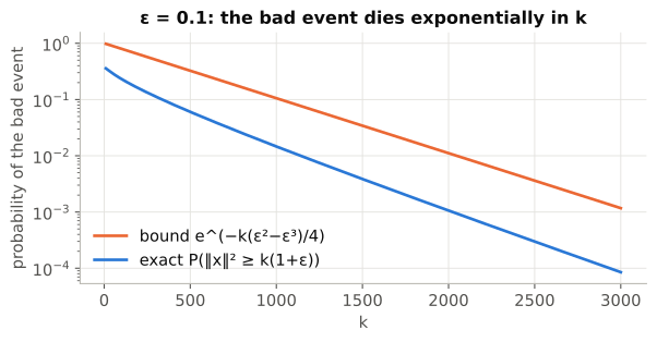
Worked example
- k = 1,000, ε = 0.1: bound .
- The exact value is 0.0146, so the bound holds.
- At k = 2,000 the bound is 0.011 and the exact value is 0.0011.
Step B: one pair fails rarely
- For one pair (x, y), take u = x − y.
- The pair is distorted by more than ε (too big or too small) with probability at most .
Step C: union bound over all pairs, which is where comes from
- There are pairs.
- By the union bound (Lesson 5),
This is less than 1 as soon as
- A failure probability below 1 means a good map exists, which is exactly what JL claims.
- If you want it to work with high probability in practice, use, for example, ; then the failure chance is at most .
Worked example: dimension requirements with explicit constants
- n = 10⁶, ε = 0.1: .
- As noted in Lesson 6, that exceeds d = 10,000.
- With d = 10⁶ (and ε = 0.2: k ≈ 3,450) the reduction is dramatic.
Does it really work? A simulation
- 200 random points in d = 10,000 dimensions, giving 19,900 pairs.
- We project with and compare every squared distance before and after.
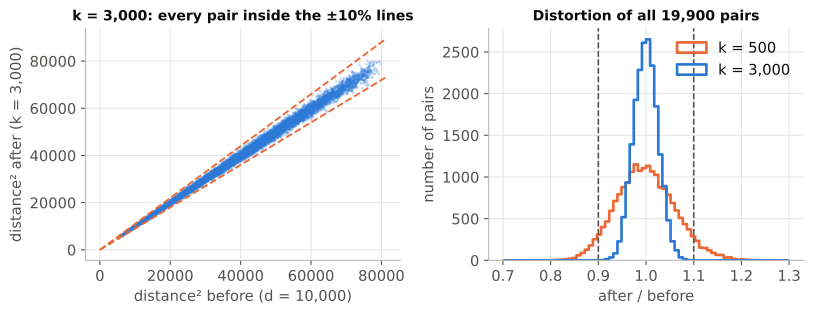
How to interpret the simulation
- In this run, k = 3,000 preserved all pairwise squared distances within the tolerance.
- The existence bound requires about 4,710 dimensions for these parameters.
- The stronger high-probability version requires about 7,060 dimensions.
- A particular dataset can succeed with fewer dimensions than a worst-case guarantee requires.
Key points to remember
- Exponentiate before applying Markov to obtain a useful tail bound.
- Control both tails, then use the union bound across all pairs.
- More target dimensions reduce the risk; stronger accuracy requires more dimensions.