SECTION 05 / 5

The SVD interpretation of random projection

On this page 8 headings

Learning goal: Understand projection as orthogonal changes of coordinates and scaling.

Conditions and notation

For the displayed k × d SVD, assume $k \leq d$ .
Squared singular values are eigenvalues of MMᵀ.
Random directions are uniform in every dimension; nearly equal singular values need a suitable dimension ratio.

The ideaSo far we treated M as a source of random measurements and estimated a length from them.
Now look at M as a machine.
The SVD uses orthogonal changes of coordinates and scaling.
For a random Gaussian M, the first rotation is random, so it can't favour any direction of your vector.
All k stretches are about equal, so nothing gets crushed.
The last rotation doesn't change length at all.
Result: the length comes out roughly unchanged.

Use this section for geometric intuition. Lessons 1 and 2 establish the probability guarantee.

Step 1: any matrix $=$ rotate · stretch · rotate

Key statement

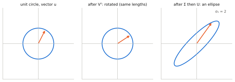
M = \frac{1}{k} R = k \times k orthonormal U k \times d "diagonal" Σ d \times d orthonormal V^{⊤}, M u = U Σ V^{⊤} u

Σ = σ_{1} ⋱ σ_{k} 0 \dots 00 (σ_{i} = singular values)

Matrices act right to left, so $M u$ happens in three steps:

$V^{⊤} u$ : rotate in $R^{d}$ . Still d numbers, same length.
Call the result $a = (a_{1}, \dots, a_{d})$ .
$Σ a$ : keep the first k coordinates, stretch them, drop the rest. $Σ a = (σ_{1} a_{1}, σ_{2} a_{2}, \dots, σ_{k} a_{k}) \in R^{k}$ .
$U (Σ a)$ : rotate in $R^{k}$ . Same length again.

Since rotations never change length, the only step that changes length is the middle one.
The exact squared-length formula is:

∥ M u ∥^{2} = ∥Σ V^{⊤} u ∥^{2} = σ_{1}^{2} a_{1}^{2} + σ_{2}^{2} a_{2}^{2} + \dots + σ_{k}^{2} a_{k}^{2} a = V^{⊤} u .

Unit circle rotated then stretched into an ellipse — In two dimensions: the unit circle is rotated (no change), then stretched by σ₁ = 2 and σ₂ = 0.5 and rotated again. It becomes an ellipse. Lengths survive only if the stretches are all close to 1 in the right sense.

Step 2: what is special about a random Gaussian M

Random rotation and scaling: the key facts

For a fixed unit input vector, the first orthogonal transformation produces a random unit direction in d dimensions.
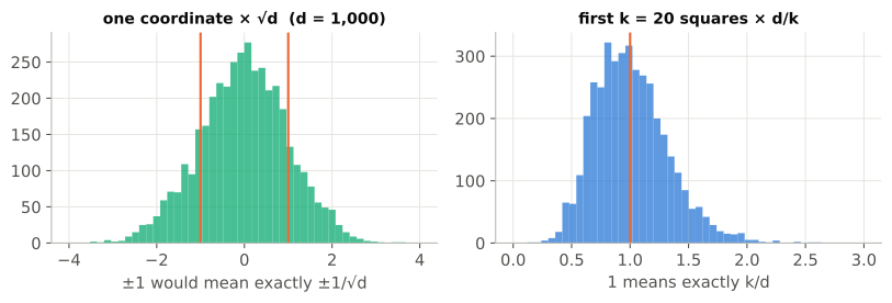
Individual coordinates fluctuate. Their squared values have expectation 1/d.
A sum of k squared coordinates is typically near k/d when k is sufficiently large.
When d is much larger than k, the nonzero singular values are near $√(d/k)$ . This is an approximation, not equality for every draw.

a=V^{\mathsf T}u,\qquad \mathbb E[a_i^2]=\frac1d

\|Mu\|^2=\sum_{i=1}^k\sigma_i^2a_i^2\approx\frac dk\sum_{i=1}^ka_i^2\approx1

The final orthogonal transformation preserves length. The probability proof works for any original dimension; a smaller target dimension is what makes projection useful.

Use d for the original dimension and k for the target dimension.
The three ideas are:

The first rotation is random. Whatever direction u points (even $(1, 0, \dots, 0)$ ), $a = V^{⊤} u$ points in a uniformly random direction.
So no coordinate is special, and $E [a_{i}^{2}] = 1/ d$ for every i (Toolkit 0.10).
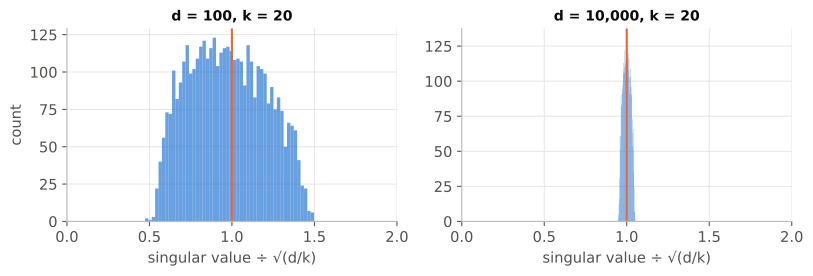
The stretches are all about $d / k$ . The sum of all squared entries of M is $σ_{1}^{2} + \dots + σ_{k}^{2}$ , and on average it equals $k \cdot d \cdot \frac{1}{k} = d$ .
Shared among k singular values, each $σ_{i}^{2} \approx d / k$ .
Random matrix theory adds that for d ≫ k they all fall in $d / k \pm 1$ .
Put together: $∥ M u ∥^{2} = \sum_{i = 1}^{k} σ_{i}^{2} a_{i}^{2} \approx \frac{d}{k} \sum_{i = 1}^{k} a_{i}^{2} \approx \frac{d}{k} \cdot \frac{k}{d} = 1$ .
The length is kept.

Histograms of singular values divided by sqrt(d/k) for d=100 and d=10000 — Singular values of $M = R / k$ , divided by $d / k$ (200 random matrices each, k = 20). With d = 100 they spread from about 0.5 to 1.5. With d = 10,000 they all sit within about ±4 % of 1. "All stretches equal" really needs d ≫ k.

One coordinate of a random unit vector vs the sum of k squared coordinates — A uniformly random unit vector in d = 1,000 dimensions. Left: a single coordinate is *not* close to ±1/√d. It is spread like a bell curve (standard deviation exactly 1/√d). Right: the sum of k = 20 squared coordinates is close to k/d (average 1.01, spread ±0.31). The heuristic only needs this right-hand fact, and its accuracy depends on k, exactly as in the proof.

Worked example: the heuristic with numbers

d = 10,000, k = 100, ‖u‖ = 1.

After the random rotation, a typical coordinate has size $1/ 10, 000 = 0.01$ , and $a_{1}^{2} + \dots + a_{100}^{2} \approx 100/10, 000 = 0.01$ .
Every singular value is $\approx 10, 000/100 = 10$ , roughly in [9, 11].
Stretched coordinates: $σ_{i} a_{i} \approx 10 \times 0.01 = 0.1 = 1/ 100$ .
$∥ M u ∥^{2} \approx 100 \times (0.1)^{2} = 1$ .
Precisely: $\approx 1 0^{2} \times 0.01 = 1$ .
The last rotation U doesn't change this.

Step 3: a random-direction experiment

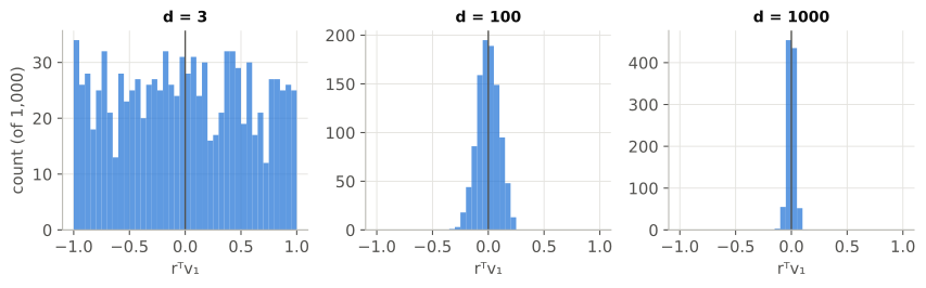
Key statementk = 2, d = 3 (then 100 or 1,000).
$M \in R^{2 \times 3}$ , $M_{ij} \sim N (0, 1) / 2$ .

Generate 1,000 such matrices; for each, $M = U Σ V^{⊤}$ , and pick the first column of V: $v_{1}, \dots, v_{1000} \in R^{3}$ , each with $∥ v_{i} ∥^{2} = 1$ .
Fix a random unit vector: $w$ with three $N (0, 1)$ entries, $r = w /∥ w ∥$ .
Compute ${r^{⊤} v_{1}, \dots, r^{⊤} v_{1000}}$ and observe this histogram.

The simulation results are shown below:

Histograms of r^T v1 for d = 3, 100, 1000 — 1,000 random matrices each. d = 3: flat over [−1, 1] (mean −0.007, standard deviation 0.578, 49 % positive). d = 100: standard deviation 0.101. d = 1,000: standard deviation 0.032. In each case the standard deviation equals $1/ d$ (0.577, 0.100, 0.032).

Check yourself

Which of the three SVD steps can change a vector's length?

Only Σ (stretching the first k coordinates and dropping the rest).
U and Vᵀ are rotations.

Why is each singular value of

R / k

about

d / k

The sum of squares of all entries is about $k d \cdot \frac{1}{k} = d$ , and that equals $\sum σ_{i}^{2}$ .
Shared among k values, each $σ_{i}^{2} \approx d / k$ .

d = 1,000,000, k = 400. Roughly what are the singular values, and the typical size of

σ_{i} a_{i}

$σ \approx 2500 = 50$ ; $a_{i} \sim 1/1000$ , so $σ_{i} a_{i} \sim 0.05 = 1/ 400$ .

True or false: the JL probability bound fails when d is small.

False.
The bound depends only on k and ε.
Small d just means there's nothing to gain from projecting.

Key points to remember

For the displayed k × d SVD, assume $k \leq d$ .
Squared singular values are eigenvalues of MMᵀ.
Random directions are uniform in every dimension; nearly equal singular values need a suitable dimension ratio.

YOUR STUDY PROGRESS

Finished this section? Save your progress.