SECTION 03 / 5

Chernoff bounds for projection error

On this page 11 headings

Learning goal: Derive an exponential upper bound on projection failure.

Conditions and notation

The ideaAdd up k squared bell-curve numbers.
The total averages k.
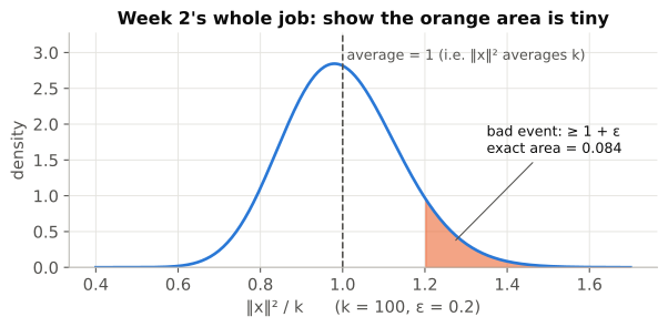
We want to show that being 20 % or more above average is extremely rare, and that it gets rarer exponentially fast as k grows.
Markov and Chebyshev are too weak for this.
The trick: before using Markov, blow the quantity up with an exponential.
This exaggerates big values so much that Markov suddenly gives a sharp answer.

Key statementn points S in $R^{d}$ are mapped by $M = \frac{1}{k} R$ to $R^{k}$ ; we want $(1 - ε) ∥ x - y ∥^{2} \leq ∥ M x - M y ∥_{2}^{2} \leq (1 + ε) ∥ x - y ∥^{2}$ for all x, y ∈ S.
For one vector u: $v = \frac{1}{k} R u$ , $E ∥ v ∥^{2} = ∥ u ∥^{2}$ , $x = \frac{k v}{∥ u ∥} \in R^{k}$ , $x \sim N (0, I)$ .

Key statement

P (bad event ∥ v ∥^{2} \geq (1 + ε) ∥ u ∥^{2}) = P (∥ x ∥^{2} \geq (1 + ε) k)

E ∥ x ∥^{2} = E [i = 1 \sum k x_{i}^{2}] = i = 1 \sum k Var (x_{i}) = 1 E [x_{i}^{2}] = k

$x \sim N (0, I)$ means $x_{1}, \dots, x_{k}$ are independent $N (0, 1)$ numbers.
For Gaussians, zero correlation (identity covariance) implies independence.
So ‖x‖² averages k, and the bad event asks for a value at least $(1 + ε)$ times its average.
Whether this is rare depends on how tightly ‖x‖² concentrates around k.
That is a concentration-inequality question.

Both inequalities apply: the squared norm is non-negative and has finite variance.
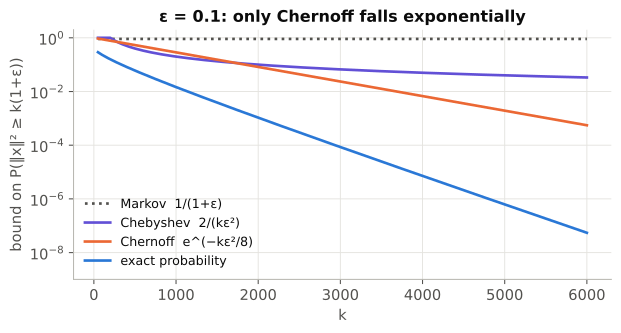
Compare the bounds they give:

Markov: $P (∥ x ∥^{2} \geq (1 + ε) k) \leq \frac{k}{( 1 + ε ) k} = \frac{1}{1 + ε}$ .
For ε = 0.1 that's 0.91, for every k.
It never improves, so it's useless.
Chebyshev: $Var (x_{i}^{2}) = E [x_{i}^{4}] - 1 = 3 - 1 = 2$ , so $Var ∥ x ∥^{2} = 2 k$ .
The bad event is a deviation of εk, so $P \leq \frac{2 k}{( ε k ) ^{2}} = \frac{2}{k ε ^{2}}$ .
That improves, but only like 1/k.

In Lesson 2 we must survive about $n^{2}$ pairs at once, so we need roughly $n^{2} \times (one-pair bound) \leq δ$ .
With Chebyshev: $n^{2} \cdot \frac{2}{k ε ^{2}} \leq δ \Rightarrow k \geq \frac{2 n ^{2}}{δ ε ^{2}}$ .
For n = 1,000, ε = 0.1, δ = 0.01 that is $k \geq 2 \times 1 0^{10}$ , far more than the original d.
We need a bound that falls exponentially in k, so that $n^{2}$ gets cancelled by a mere log.

Chernoff-style boundFor any λ > 0:

P (∥ x ∥^{2} \geq (1 + ε) k) = P (e^{λ ∥ x ∥^{2}} \geq e^{λ (1 + ε) k}) \leq \frac{E [ e ^{λ ∥ x ∥^{2}} ]}{e ^{λ (1 + ε) k}} (Markov) = \frac{E [ e ^{λ \sum_{i = 1}^{k} x_{i}^{2}} ]}{e ^{λ (1 + ε) k}}

The equality: $t \mapsto e^{λ t}$ is increasing for λ > 0, so the two events are the same event (Toolkit 0.2).
The inequality: Markov's inequality, $P (Y \geq a) \leq E [Y] / a$ , applied to the non-negative random variable $Y = e^{λ ∥ x ∥^{2}}$ with $a = e^{λ (1 + ε) k}$ .
Why bother? The exponential makes big values of ‖x‖² count enormously, so Markov's single number $E [Y]$ "feels" the whole tail.
And the exponential turns the sum into a product of independent pieces, which we can compute exactly.

Key statement

= \frac{E [ e ^{λ x_{1}^{2} + λ x_{2}^{2} + \dots + λ x_{k}^{2}} ]}{e ^{λ (1 + ε) k}} = \frac{E [ \prod _{i = 1}^{k} e ^{λ x_{i}^{2}} ]}{e ^{λ (1 + ε) k}} = \frac{\prod _{i = 1}^{k} E [ e ^{λ x_{i}^{2}} ]}{e ^{λ (1 + ε) k}} = \frac{\prod _{i = 1}^{k} \frac{1}{1 - 2 λ}}{e ^{λ (1 + ε) k}}

P (bad event) \leq (\frac{1}{1 - 2 λ})^{k /2} / e^{λ (1 + ε) k} .

$e^{a + b} = e^{a} e^{b}$ : the sum in the exponent becomes a product.
The $x_{i}$ are independent, so the expectation of the product is the product of expectations (Toolkit 0.3).
Each factor is the Gaussian MGF fact $E [e^{λ Z^{2}}] = 1/ 1 - 2 λ$ (Toolkit 0.4).
The same factor appears k times, giving the power k/2.

Key statement

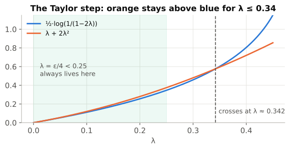
= exp (lo g (\frac{1}{1 - 2 λ})^{k /2} - λ (1 + ε) k) = exp (k [\frac{1}{2} lo g \frac{1}{1 - 2 λ} - λ (1 + ε)])

\leq exp (k (λ + 2 λ^{2} - λ - λ ε)) = exp (k (2 λ^{2} - λ ε))

(Taylor series of log, small enough λ)

f (λ) = 2 λ^{2} - λ ε, f^{'} (λ) = 4 λ - ε = 0 \Rightarrow λ = \frac{ε}{4}

f (\frac{ε}{4}) = \frac{2 ε ^{2}}{16} - \frac{ε ^{2}}{4} = - \frac{ε ^{2}}{8} ⟹ P (bad) \leq exp (k (- \frac{ε ^{2}}{8}))

Rewrite as one exponential: $y = e^{l o g y}$ , and bring the denominator up as a minus sign in the exponent.
Then pull out k.
Taylor step: $\frac{1}{2} lo g \frac{1}{1 - 2 λ} \leq λ + 2 λ^{2}$ for small λ (valid up to λ ≈ 0.342, Toolkit 0.5).
The two λ terms cancel, leaving a simple parabola.
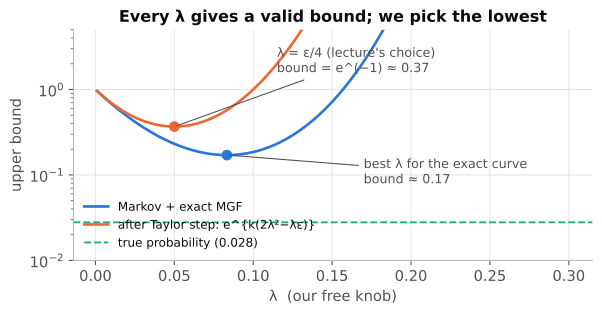
Choose λ: every allowed λ gives a valid upper bound, so we pick the one that makes the bound smallest.
The parabola's bottom is at λ = ε/4 (Toolkit 0.6).

k = 200, ε = 0.2.

Bad event: $∥ x ∥^{2} \geq 1.2 \times 200 = 240$ , while the average is 200.
λ = ε/4 = 0.05.
MGF factor: $1/ 1 - 0.1 = 1.0541$ ; to the power 200: $(1/0.9)^{100} = e^{10.536}$ .
Denominator: $e^{0.05 \times 240} = e^{12}$ .
Markov + exact MGF: $e^{10.536 - 12} = e^{- 1.464} \approx 0.231$ .
After the Taylor step: $e^{200 (2 \times 0.0025 - 0.05 \times 0.2)} = e^{200 \times (- 0.005)} = e^{- 1} \approx 0.368$ , which equals $e^{- k ε^{2} /8} = e^{- 200 \times 0.04/8}$ . ✓
True probability (computed exactly from the chi-square distribution): 0.028.
The bound holds.

ε = 0.1, so the bound is $e^{- k /800}$ : k = 1,000 gives 0.29; k = 2,000 gives 0.082; k = 5,000 gives 0.0019; k = 10,000 gives $3.7 \times 1 0^{- 6}$ .
Each extra 1,000 dimensions multiplies the bound by the same factor $e^{- 1.25} \approx 0.29$ .

Why can we apply Markov to

e^{λ ∥ x ∥^{2}}

It's never negative (an exponential is always positive), which is all Markov needs.

Where exactly is independence used?

To turn $E [\prod_{i} e^{λ x_{i}^{2}}]$ into $\prod_{i} E [e^{λ x_{i}^{2}}]$ .

Evaluate the bound

e^{- k ε^{2} /8}

for k = 400, ε = 0.2.

$e^{- 400 \times 0.04/8} = e^{- 2} \approx 0.135$ .

If ε halves, how must k change to keep the same bound?

The exponent is kε²/8, so k must become 4×.

YOUR STUDY PROGRESS

Finished this section? Save your progress.